The viz reference

Every function orbix.viz exports, with the smallest call that produces a real picture. This page is a reference rather than a walkthrough: it is organized by function, not by task, so it answers “what does this one draw?” For the narrative version, which builds a figure up argument by argument, see Plotting orbits.

Every figure below is executed when these docs are built, on seeded synthetic data and nothing else, so a function that stops rendering fails the build rather than the documentation host.

import hwostyle
import matplotlib
import jax.numpy as jnp
import numpy as np
import eyepiece as ep

from orbix import KeplerianOrbit
from orbix import viz

hwostyle.use("dark")

# Docs-builder concerns, not lines to copy into your own scripts. hwostyle asks
# for Inter/Helvetica/Arial and a CI builder has none of them, so name the face
# matplotlib always ships as a last resort -- otherwise every figure emits a
# findfont warning. And render at a resolution that holds up on a high-DPI
# screen; the notebook default of 100 dpi does not.
matplotlib.rcParams["font.sans-serif"] = list(
    matplotlib.rcParams["font.sans-serif"]
) + ["DejaVu Sans"]
matplotlib.rcParams["figure.dpi"] = 160

MSUN_KG = 1.988409870698051e30
styles = ep.SourceStyles(["planet b", "planet c", "planet d"])

# One eccentric, inclined orbit carries most of this page. Its elements are
# named here because the posterior fan further down is built around them.
A_AU, ECC, INC_RAD = 1.3, 0.31, 1.05
BIG_OMEGA_RAD, SMALL_OMEGA_RAD, M0_RAD = 2.3, -0.7, 0.4
T0_D = 2460000.0

# Kepler's third law for a solar-mass star, so the track below can span
# exactly one period and close on itself.
PERIOD_D = A_AU**1.5 * 365.25
PERIAPSIS_D = T0_D - M0_RAD * PERIOD_D / (2.0 * np.pi)

orbit = KeplerianOrbit(
    a_AU=A_AU, e=ECC, W_rad=BIG_OMEGA_RAD, i_rad=INC_RAD,
    w_rad=SMALL_OMEGA_RAD, M0_rad=M0_RAD, t0_d=T0_D,
)
t_jd = jnp.linspace(T0_D, T0_D + PERIOD_D, 240)

# A second cast for the 3D views: three near-coplanar planets, the way a
# planetary system actually sits. Keeping the mutual inclinations small (7 to
# 16 degrees) keeps the z excursion to about a quarter of the in-plane extent,
# so the orbits read as nested ellipses seen from above rather than as thin
# slivers pointed at the camera.
PLANETS = ["planet b", "planet c", "planet d"]
SYS_A_AU = np.array([0.72, 1.30, 2.35])
SYS_ECC = np.array([0.05, 0.21, 0.40])
SYS_BIG_OMEGA = np.array([2.20, 2.35, 2.50])
SYS_INC = np.array([0.12, 0.20, 0.28])
SYS_SMALL_OMEGA = np.array([-0.40, -0.70, 0.90])
SYS_M0 = np.array([0.00, 2.10, 4.30])

system = KeplerianOrbit(
    a_AU=SYS_A_AU, e=SYS_ECC, W_rad=SYS_BIG_OMEGA, i_rad=SYS_INC,
    w_rad=SYS_SMALL_OMEGA, M0_rad=SYS_M0, t0_d=np.full(3, T0_D),
)

# The same three planets one at a time. plot_orbit applies a single style to
# every track it is handed -- a fan of draws for one planet is one source -- so
# giving each planet its own colour means one call per planet.
one_planet = [
    KeplerianOrbit(
        a_AU=SYS_A_AU[k:k + 1], e=SYS_ECC[k:k + 1],
        W_rad=SYS_BIG_OMEGA[k:k + 1], i_rad=SYS_INC[k:k + 1],
        w_rad=SYS_SMALL_OMEGA[k:k + 1], M0_rad=SYS_M0[k:k + 1],
        t0_d=np.array([T0_D]),
    )
    for k in range(3)
]

OUTER_PERIOD_D = 2.35**1.5 * 365.25
t_system = jnp.linspace(T0_D, T0_D + OUTER_PERIOD_D, 240)

plot_sky_track

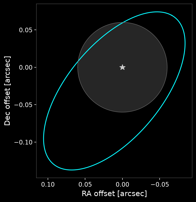
The sky-plane track in arcseconds: RA offset increasing to the left per the astronomical convention, Dec offset up, the star at the origin, equal aspect. iwa shades the inner working angle a coronagraph cannot see into.

result = viz.plot_sky_track(
    orbit, t_jd, Ms_kg=MSUN_KG, dist_pc=10.0,
    style=styles["planet b"], iwa=0.06,
)

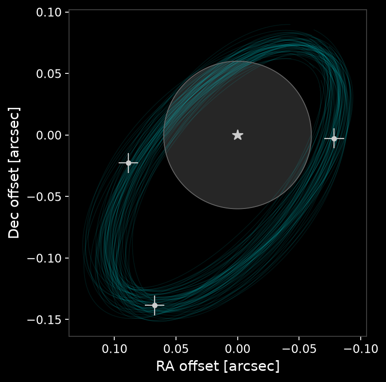
The same function draws a (K,)-batched orbit as a fan of candidates faded by weight, which is what a posterior looks like. data overlays measured epochs as points with error bars.

rng = np.random.default_rng(11)
# The measured epochs come FROM the orbit above, perturbed by the measurement
# error -- otherwise the figure shows a posterior next to data it disagrees
# with, which is exactly the thing a fan is supposed to rule out.
SIGMA_ARCSEC = 0.008
t_obs = T0_D + np.array([70.0, 250.0, 430.0])
ra_true, dec_true = orbit.position_arcsec(
    t_jd=jnp.asarray(t_obs), Ms_kg=MSUN_KG, dist_pc=10.0
)
epochs = (
    np.asarray(ra_true)[0] + SIGMA_ARCSEC * rng.standard_normal(3),
    np.asarray(dec_true)[0] + SIGMA_ARCSEC * rng.standard_normal(3),
    np.full(3, SIGMA_ARCSEC),
)

# ... and the fan is a posterior scattered around that same orbit.
K = 60
fan = KeplerianOrbit.from_period(
    T_d=PERIOD_D * (1.0 + 0.04 * rng.standard_normal(K)),
    e=np.clip(ECC + 0.04 * rng.standard_normal(K), 0.0, 0.9),
    cos_i=np.clip(np.cos(INC_RAD) + 0.06 * rng.standard_normal(K), -1.0, 1.0),
    W_rad=BIG_OMEGA_RAD + 0.08 * rng.standard_normal(K),
    cos_w=np.cos(SMALL_OMEGA_RAD + 0.15 * rng.standard_normal(K)),
    sin_w=np.sin(SMALL_OMEGA_RAD + 0.15 * rng.standard_normal(K)),
    tp_d=PERIAPSIS_D + 12.0 * rng.standard_normal(K),
    Ms_kg=MSUN_KG,
)
weights = rng.dirichlet(np.full(K, 3.0))
result = viz.plot_sky_track(
    fan, t_jd, Ms_kg=MSUN_KG, dist_pc=10.0,
    style=styles["planet b"], weights=weights, iwa=0.06, data=epochs,
)

Bare arrays work anywhere an orbit does, so tracks loaded from a file draw through the same door: viz.plot_sky_track((ra, dec)).

plot_orbit

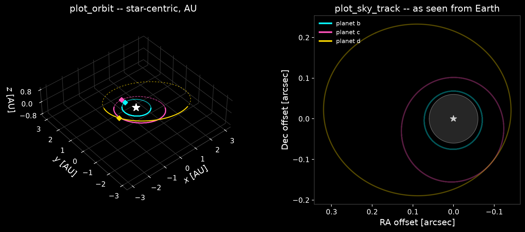
The star-centric orbits in three dimensions, in AU, through eyepiece.trail, shown next to the same system on the sky so the two doors can be read against each other. SourceStyles is what ties them together: each planet keeps its colour across both panels, so the yellow ring 2.35 AU out in the left panel is the yellow ring reaching 0.24 arcsec in the right one. That is the whole point of the eyepiece identity helpers, and it is worth more here than any single view.

The two panels tell you different things. The left one shows the geometry the star sees: three near-coplanar orbits, nested, with the outer planet’s eccentricity visible as the star sitting off centre. The right one shows the geometry the telescope sees, in arcseconds, with the inner working angle that decides what is observable at all.

Point the 3D camera down on the system’s own plane rather than at its edge. The default 3D view sits 79 degrees off an orbit normal like this one, which squashes an ellipse to a fifth of its width and reads as a sliver aimed at the viewer; elev=42, azim=-130 is open enough to read and still far enough from face-on for the depth cue to work. marks adds the exact periapsis as a diamond in each planet’s own colour.

Set the camera before calling: the per-point depth cue on a still is baked from the camera at call time, so a view_init afterwards moves the scene without moving the cue. That is also why this page creates the 3D axes by hand here rather than letting the function do it.

import matplotlib.pyplot as plt
from matplotlib.lines import Line2D
from matplotlib.ticker import MaxNLocator

fig = plt.figure(figsize=(11.5, 4.8), layout="constrained")
gs = fig.add_gridspec(1, 2, width_ratios=[1.25, 1.0])
ax3d = fig.add_subplot(gs[0], projection="3d")
ax3d.view_init(elev=42.0, azim=-130.0)
axsky = fig.add_subplot(gs[1])

for name, planet in zip(PLANETS, one_planet):
    viz.plot_orbit(
        planet, t_system, Ms_kg=MSUN_KG, ax=ax3d,
        style=styles[name], marks={"periapsis"},
    )

# plot_orbit sizes the 3D box as a cube. That is right for a steep orbit, but a
# near-coplanar system then leaves about three quarters of the height empty.
# Shrinking the z limit and the box aspect by the SAME factor fills the frame
# and keeps the scale equal on all three axes; the tick locator keeps the
# shorter axis from crowding its labels together.
z_half = 1.15 * float(np.max(np.abs(
    np.asarray(system.propagate(t_jd=t_system, Ms_kg=MSUN_KG)[0])[:, 2]
)))
xy_half = ax3d.get_xlim()[1]
ax3d.set_zlim(-z_half, z_half)
ax3d.set_box_aspect((1.0, 1.0, z_half / xy_half))
ax3d.zaxis.set_major_locator(MaxNLocator(3))
ax3d.set_title("plot_orbit -- star-centric, AU")

viz.plot_sky_track(
    system, t_system, Ms_kg=MSUN_KG, dist_pc=10.0, ax=axsky,
    colors=[styles[name]["color"] for name in PLANETS], iwa=0.06,
    fan_kw={"lw": 1.8},
)
axsky.set_title("plot_sky_track -- as seen from Earth")
axsky.legend(
    handles=[Line2D([], [], color=styles[n]["color"], lw=2.5, label=n)
             for n in PLANETS],
    loc="upper left", frameon=False, fontsize=9,
)

<matplotlib.legend.Legend at 0x7b8a0e959820>

animate_orbit

Returns a lazy eyepiece.Animation: nothing renders until a sink is asked for, and one animation feeds several sinks in a single draw pass (.save("orbit.mp4", "orbit.gif")). Here it goes to jshtml, which needs no ffmpeg and so survives any documentation builder.

kind="3d" gives the star-chart presentation, kind="sky" the sky-plane track. history controls the trail: "all" accumulates, an integer keeps a trailing window, "none" moves the heads alone.

rotate controls the camera sweep. A dict of (start_deg, stop_deg) pairs gives full manual control, and any axis left out is held at its current value, so the call below is a single-axis azimuth sweep with elevation pinned.

Where you put that sweep still matters. The projected area of a planar ellipse is pi * a * b * cos(tilt), with tilt measured to the orbit normal, so an azimuth sweep that changes the tilt changes the drawn size and the orbits read as inflating rather than turning. A near-coplanar system makes this easy, because its normal is only 14 degrees off the rotation axis: centred on that normal’s own azimuth the window below holds the drawn size to 1.02x, where a window placed a quarter turn away gives 1.18x. Elevation 46 leaves the camera 58 degrees off the normal, far enough from face-on that the depth cue still reads across the outer planet (0.07 to 0.93 of full scale). rotate="auto" sidesteps the placement question by travelling a cone about the orbit normal at fixed tilt, which holds the size exactly but moves azimuth and elevation together; None holds the camera still.

from IPython.display import HTML

t_anim = jnp.linspace(T0_D, T0_D + OUTER_PERIOD_D, 72)

anim = viz.animate_orbit(
    system, t_anim, Ms_kg=MSUN_KG, kind="3d", history="none",
    base_ms=viz.size_by_radius([1.0, 3.9, 11.2]), fps=15,
    rotate={"azim": (-150.0, -110.0), "elev": (46.0, 46.0)},
)
HTML(anim.jshtml(dpi=130))

Once Loop Reflect

The same plot, different options

Each function above takes the same data and renders it several ways. These matrices vary one argument at a time so the effect of each is visible on its own, rather than described.

plot_sky_track on one posterior fan, one option added per panel:

# Three colours from ONE SourceStyles: a fresh SourceStyles restarts the
# palette, so asking for three separate ones would give the same colour thrice.
families = ep.SourceStyles(["alias A", "alias B", "alias C"])
per_track = [families[f"alias {c}"]["color"] for c in "ABC"] * (len(weights) // 3)

# Deliberately lumpy weights; a near-uniform posterior fades almost invisibly.
lumpy = np.random.default_rng(3).dirichlet(np.full(len(weights), 0.35))

variants = [
    ("plot_sky_track(fan, ...)", {}),
    ("weights=posterior_mass", {"weights": lumpy}),
    ("colors=per_track", {"colors": per_track}),
    ("iwa=0.06", {"iwa": 0.06}),
    ("data=(ra, dec, err)", {"data": epochs}),
    ("invert_ra=False", {"invert_ra": False}),
]
fig, axes = plt.subplots(2, 3, figsize=(12.0, 7.4), layout="constrained")
for ax, (label, kw) in zip(axes.ravel(), variants):
    viz.plot_sky_track(
        fan, t_jd, Ms_kg=MSUN_KG, dist_pc=10.0, ax=ax,
        style=styles["planet b"], **kw,
    )
    ax.set_title(label, fontsize=10.5)

plot_orbit on the same system. With no style it uses the star-chart look – markers in the mode’s text colour over a transparent dashed grey path – and style= opts into a source’s solid colour instead:

fig, axes = plt.subplots(
    1, 3, figsize=(12.6, 4.2), layout="constrained",
    subplot_kw={"projection": "3d"},
)
orbit_variants = [
    ("star-chart default", {}),
    ("style=", {"style": styles["planet b"]}),
    ("marks={'periapsis', 'nodes'}",
     {"style": styles["planet b"], "marks": {"periapsis", "nodes"}}),
]
for ax, (label, kw) in zip(axes, orbit_variants):
    ax.view_init(elev=42.0, azim=-130.0)
    viz.plot_orbit(system, t_system, Ms_kg=MSUN_KG, ax=ax, **kw)
    ax.set_title(label, fontsize=10.5)

And the trail. history decides how much of the path behind each planet stays drawn, which is the difference between a plot that reads as motion and one that reads as a snapshot. Note that this only shows up against a solid style: under the star-chart default the trail is the same dim grey as the ghost path and the three settings look identical.

animate_orbit builds its own figure and takes no ax, unlike the static functions, so these three frames are rendered separately and tiled:

import io

frames = []
for history in ["all", 15, "none"]:
    anim = viz.animate_orbit(
        system, t_system[::4], Ms_kg=MSUN_KG, kind="3d", history=history,
        rotate=None, style=styles["planet b"],
        base_ms=viz.size_by_radius([1.0, 3.9, 11.2]),
    )
    for i, frame in enumerate(anim.frames):
        anim.draw(frame, i)
        if i == 44:
            break
    buf = io.BytesIO()
    anim.fig.savefig(buf, format="png", bbox_inches="tight", dpi=150)
    plt.close(anim.fig)
    buf.seek(0)
    frames.append(plt.imread(buf))

fig, axes = plt.subplots(1, 3, figsize=(12.6, 4.4), layout="constrained")
for ax, image, label in zip(axes, frames,
                            ['history="all"', "history=15", 'history="none"']):
    ax.imshow(image)
    ax.set_axis_off()
    ax.set_title(label, fontsize=10.5)

size_by_radius

Marker diameters from planet radii, interpolated geometrically between Mercury and Jupiter by default. The resting marker size is the anchor the depth cue swells around, so it is the place physical meaning belongs.

names = ["Mercury", "Earth", "Neptune", "Jupiter"]
radii = [0.38, 1.0, 3.9, 11.2]

# One vectorized call: the result is always an array of shape (K,), so a
# scalar radius comes back as a one-element array rather than a float.
for name, r_earth, ms in zip(names, radii, viz.size_by_radius(radii)):
    print(f"{name:8s} {r_earth:5.2f} R_earth -> {ms:5.2f} pt")

Mercury   0.38 R_earth ->  3.00 pt
Earth     1.00 R_earth ->  4.11 pt
Neptune   3.90 R_earth ->  6.39 pt
Jupiter  11.20 R_earth ->  9.00 pt

The result is a set of marker diameters, which is what animate_orbit(base_ms=...) takes. Do not hand it to plot_orbit(marker_scale=...): that reaches scatter(s=...), an area, so the encoding would be silently square-rooted.

depth_scale and depth_size

The two halves of the depth cue, public so a caller can reproduce it on their own artist. depth_scale turns positions and a camera into a factor in [0, 1] – 0 at the far side of the orbit, 1 at the near side. depth_size maps that factor onto a marker-diameter multiplier.

Positions are (N, 3), one row per point, while propagate returns (K, 3, N); transpose one orbit out of the batch to feed it.

xyz = np.asarray(orbit.propagate(t_jd=t_jd, Ms_kg=MSUN_KG)[0][0]).T
depth = viz.depth_scale(xyz, azim_deg=-50.0, elev_deg=25.0)
mult = viz.depth_size(depth)

print(f"depth  in [{depth.min():.2f}, {depth.max():.2f}]")
print(f"marker in [{mult.min():.3f}, {mult.max():.3f}] x base")

depth  in [0.01, 0.99]
marker in [1.002, 1.223] x base

Both return plain arrays rather than figures, so this last picture is drawn with bare matplotlib. There is no eyepiece primitive for a mapping curve and there should not be: a primitive that wrapped ax.plot would be reimplementing matplotlib, not adding anything.

fig, (ax1, ax2) = plt.subplots(1, 2, figsize=(9.0, 3.2), layout="constrained")

ax1.plot(depth, lw=1.5)
ax1.set_xlabel("epoch index along the orbit")
ax1.set_ylabel("depth factor")
ax1.set_title("depth_scale along the track")

grid = np.linspace(0.0, 1.0, 200)
ax2.plot(grid, viz.depth_size(grid), lw=1.5)
ax2.set_xlabel("depth factor")
ax2.set_ylabel("diameter multiplier")
ax2.set_title("depth_size, peaking at +22%")

Text(0.5, 1.0, 'depth_size, peaking at +22%')

The far side is the anchor at exactly the base size and the near side swells by about a fifth, so depth reads as a brief swell rather than a shrink, and the resting size stays free to mean something physical.